Visual and Data Analysis - FIFA 19

Data Science project to analyze and discover insights of the attributes of each player registered in the latest edition of FIFA 19 database. Most of the project was done with Jupyter Notebook, so that the reader can see and understand the code implemented.

Table of Contents

• Data
• Performed Analysis
• Insights
• Technologies and Techniques
• Python Libraries
• Contributing and Feedback
• Author
• License

Data

Detailed attributes for every player registered in the latest edition of FIFA 19 database:

• Original data from Kaggle
• Project data in GitHub

Performed Analysis

1. Exploration and Profiling
2. Querying Data
3. Principal Component Analysis
4. Clustering Data - KMeans
5. Analysis of Similarity
6. Networks and Force System

Insights

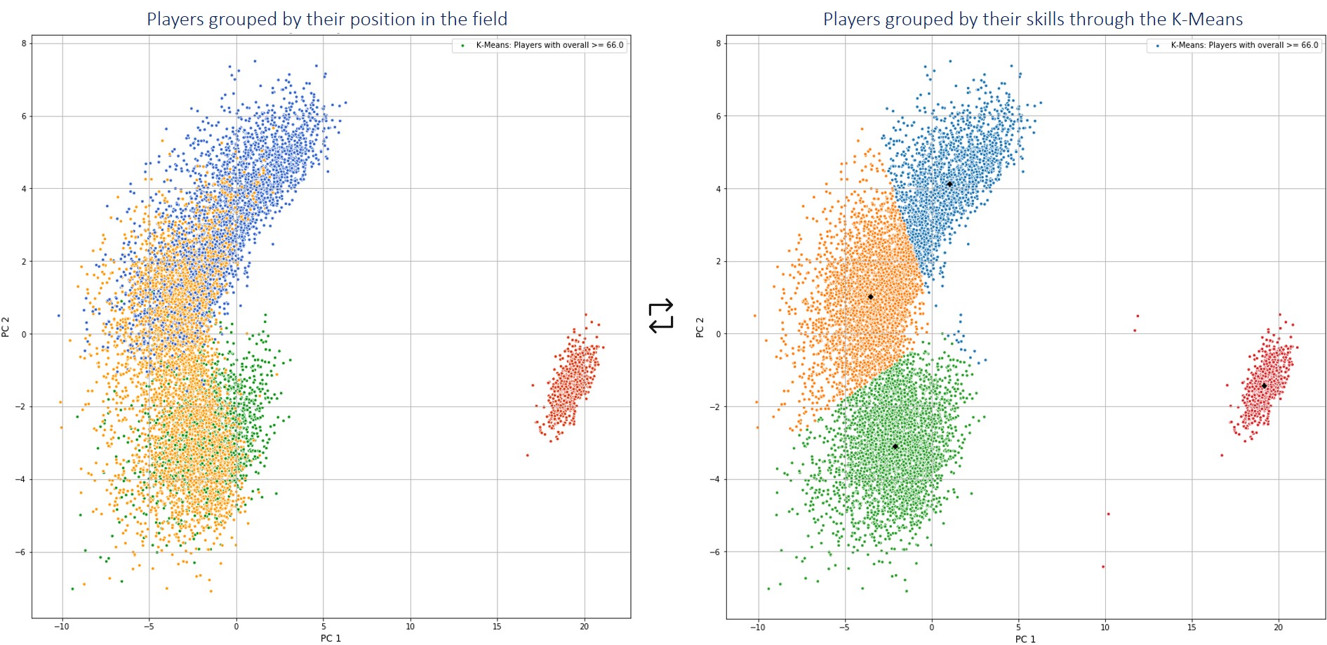
• With these data it is possible to perform a PCA of the skills of the players and maintain 80.5% of the variance of the data with only 2 components. Which allows us to plot the players on the plane and analyze which players resemble each other.
• The similarity between players is better identified with 2 components (2D plot and 80.5% variance explained) than with 3 components (3D plot and 84.8% variance explained).
• Using the Jambu elbow technique, you can visually select the optimal value of k = 4 (number of clusters between which the data will be grouped).
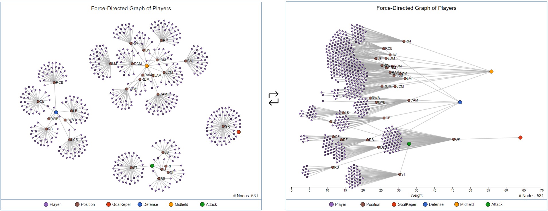
• Players can be grouped into 4 groups. These groups are highly related to the zones in which players play on the field (goalkeepers, defenders, midfielders and strikers).
• You can calculate the N players most similar to a specific player, using the similarity functions.
• The matrix of correlation by individuals allows to see the correlation that exists between the players. It is the same item-item approach of the recommendation systems.
• Others:
  • The team with the most potential is FC Barcelona, whose players initially have an overall average of 78 but can reach 85.
  • The player with the most potential is MBappe from PSG, who can reach 95 of overall.
  • However, the player with the most improvement margen is Donnarumma of AC Milan, who initially has an overall of 82 but can reach 93 (+11).
  • The PCA was succeeded because there are a great number of correlated variables in the original dataset. This allowed the eigenvector to be significant.
  • There is a large number of correlated variables in the original dataset, which is an ideal scenario to run a PCA and thus reduce the dimensions while maintaining the variance and the direction of the data.

Technologies and Techniques

• Python 3.6.8
• Anaconda Navigator 1.9.7
• Jupyter Notebook 5.7.8
• Force System of d3.js
• Principal Component Analysis (PCA)
• K-Means

Python Libraries

• pandas
• pandas_profiling
• numpy
• pandasql
• stats
• sklearn
• sklearn.metrics.pairwise
• StandardScaler
• PCA
• KMeans
• matplotlib.pyplot
• mpl_toolkits.mplot3d
• seaborn
• ipywidgets

Python Dependencies

  conda install -c conda-forge pandas-profiling

Contributing and Feedback

Any kind of feedback/suggestions would be greatly appreciated (algorithm design, documentation, improvement ideas, spelling mistakes, etc…). If you want to make a contribution to the course you can do it through a PR.

Author

• Created by Andrés Segura Tinoco
• Created on May 1, 2019
• Updated on Setp 14, 2021

License

This project is licensed under the terms of the MIT license.